A Scientific Risk Limit System for A Crypto Futures

The below insightful new article penned by KuCoin’s founder, Michael Gan, and Head of Derivatives, Ken Tian, delves into the innovative backend logic of KuCoin’s new risk limit system for cross-margin, similar to traditional finance, showcasing KuCoin’s commitment to technical excellence and robust risk management strategies.

Introduction

Many cryptocurrency exchanges adopt complex risk management measures to prevent liquidation risks. These include setting multi-level risk limits and restricting the use of high leverage. Additionally, exchanges dynamically adjust parameters like risk limits and margin rates based on the underlying asset’s price and market liquidity. However, these processes are not only complex but also lack clear management standards, requiring significant resources to maintain a system that may not be internally consistent—for example, increasing capital may not allow for larger positions due to abrupt changes in leverage tiers.

On some trading platforms (see Figure 1), there are nearly a hundred risk limit tiers. These passive tier changes increase the complexity of system management and can result in partial forced liquidation, undermining users’ interests.

We aim to develop a nonlinear model to simulate reasonable position sizes for a given capital, enabling more flexible and efficient risk management. This approach involves rebuilding the internal formula system to achieve self-consistency, providing a viable alternative to the existing complex risk limit templates.

This paper proposes a new risk management framework as a replacement for the current limit models. The new approach has already been implemented in KuCoin’s cross-margin system, exhibiting some obvious advantages:

1. It is closer to the position management settings used by traditional exchanges, making it easier for institutional capital to adapt.
2. It eliminates the need to adjust risk limits based on position size or leverage usage.
3. It simplifies operational processes, reducing the burden on the exchange while mitigating the risk of harming users’ interests to protect the exchange’s own benefits.

This model provides a more transparent and streamlined approach to risk management, aligning both exchange operations and user interests.

The model

Maximum Position Size

We assume that a user’s account holds capital C, and the price of the underlying asset’s futures contract is p. The initial margin rate r corresponds to the reciprocal of the leverage selected by the user. Ignoring transaction fees, the number of contracts the user can open is given by:

N = C/(p ∗ r)

However, if the capital C is too large or the margin rate r is too low, the associated risks for the exchange become significant. Therefore, when both C and rrr are fixed and C is large, the maximum allowable position will be limited by the exchange’s risk tiers to much less than C/(p*r). Conversely, with smaller capital C, the position size can approach C/(p*r).

Many exchanges implement dozens to hundreds of risk tiers to manage this relationship. As a result, users frequently need to adjust their tier level as their capital grows. The objective behind these restrictions can be roughly expressed using a logarithmic function:

N = ln(C/(p ∗ r) + 1)

Clearly, when C is large, the first derivative of the logarithmic function decreases, meaning the achievable position size will be smaller than that calculated by a linear formula. However, this presents a challenge: for the approximation ln(x+1)≈x to hold, C must be sufficiently small, and p must be large. Otherwise, even with small C, users may still be unable to achieve the theoretical maximum position size of C/(p*r).

To address this, we need to introduce a larger scaling parameter k based on the characteristics of different contract types. The original equation is then modified as follows:

N = k ∗ ln(C/(p ∗ r ∗ k) + 1)

This adjustment satisfies the needs of small-capital users while also meeting the risk control requirements for large-capital users.

To take into account open positions and other margin requirements in KuCoin’s cross-margin system, let’s define the following:

• F: Margin occupied by other contracts and open orders.
• E: Total equity in the user’s futures account.
• Q: Position size of pending orders aligned with the same direction as the new order.
• O: Current open position size (positive if aligned with the new order, negative if in the opposite direction).

The equation for calculating the maximum allowable position is then:

N = max(0, k ∗ ln((E − F )/(k ∗ p ∗ r) + 1) − Q − O)

Therefore, under this model on KuCoin, for capital of a typical size, the relationship between leverage and the maximum allowable position can be visualized as follows:

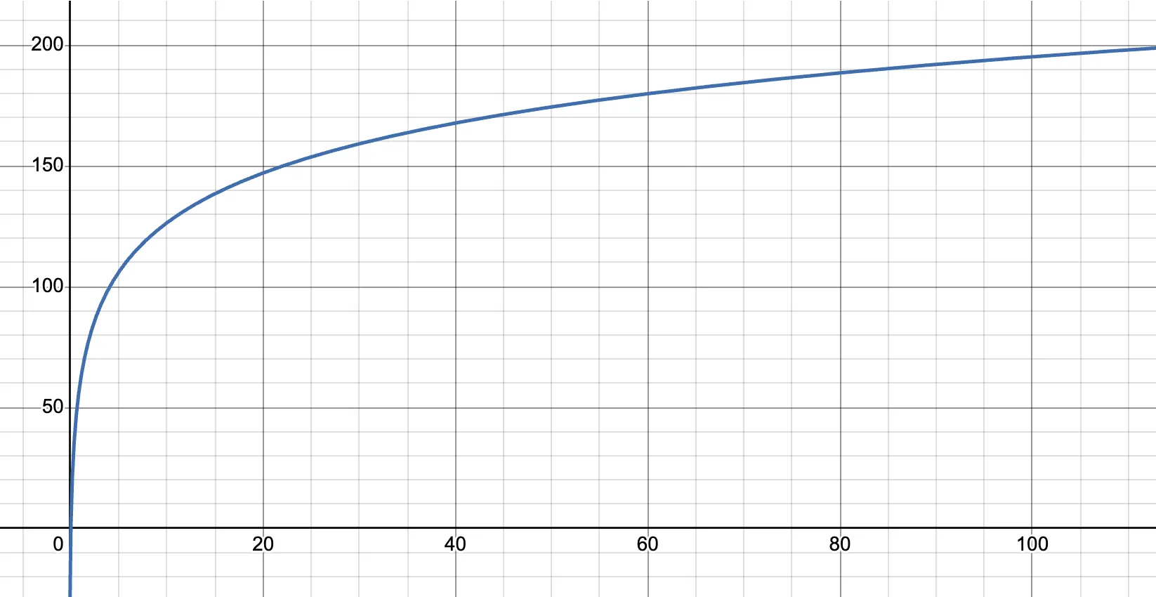
This chart reflects how the model ensures scalability and stability, balancing between the needs of smaller users (to maximize position size) and risk control for larger users through nonlinear margin adjustments.

However, on most exchanges (such as OKX and Binance), the relationship between leverage and position size often follows a distorted curve:

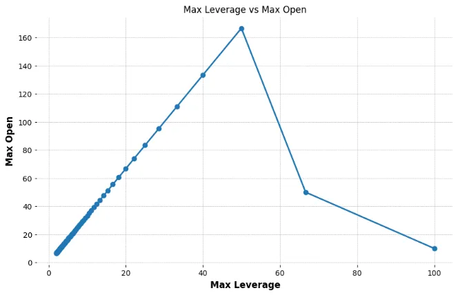
In fact, even MMR (Maintenance Margin Rate) follows a similar pattern. This can be particularly challenging for large-capital users. For example, when the IMR (Initial Margin Rate) is set at 50%, the MMR might be as high as 48%. In such cases, users attempting to open large positions are restricted to using low leverage, but the MMR is increased to an unreasonable extent.

This setup limits users’ ability to effectively utilize their capital, as leverage tiers shift abruptly and require frequent adjustments, reducing flexibility. It creates an imbalance between risk management and user experience, making it difficult for large investors to operate efficiently within these constraints.

MMR and IMR

The MMR (Maintenance Margin Rate) essentially serves as a compensation mechanism for the exchange to manage liquidation risks. At its core, MMR reflects the pressure on liquidity extraction and needs to adjust dynamically with changes in open positions. Below, we derive the theoretical value of MMR based on liquidity-related metrics available to the exchange.

Liquidity-Related Variables

To properly assess liquidity, the following variables are identified, which are typically accessible to exchanges:

• μ: Speed of market order execution
• T: Time requirement for liquidation or trading
• i: Price/level distance from the best bid or askj: Ticker time unit
• Qi: Average number of orders at a distance iii from the order book
• S: Average size of an order (with SmS_mSm for market orders, SlS_lSl for limit orders)
• N: Number of orders (with Nm for market orders, Nc for cancellations, and Ni for limit orders)

These values represent the average conditions in a stable market.

Defining User Position Metrics

• position: Instantaneous average position size of all users, which can come from the exchange’s empirical values.
• pos: position size held by any user
• X: Sum of the traded volume within MMR levels over the trading period
• MMRup: Upper limit for MMR
• rMMR: Final value of the MMR
• R: actual distance from best bid or ask, not the same as r, often depends on i, j

Adjustment of MMR with Order Flow

The speed of limit order entries and cancellations is included as part of the average over multiple levels. Given that market orders are more likely to execute instantly, we need to account for this relative increase or decrease. The following relationships define the dynamics:

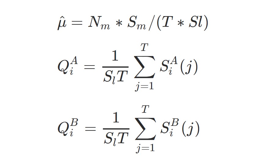
For example, taking a long position, the corresponding strong liquidation liquidity can be the buy order quantity (Q):

For exchange’s security, we get:

X(R) = position R = f (position)
R = f (position)

Here, it is not far to reach that position and R have an approximately inverse relationship. And for minimum order quantity:

R = p × MMR

The position is known, given the constraint relationships of variables. MMR is independent of p, so:

MMR = g(position) = z(Q, S, T , μ^, i, j) = f(position)/p

Therefore, the final value of rMMR can be expressed as:

rMMR = min(MMRup, MMR)

From the above equations, it can be seen that, apart from R, other variables such as position, Q, S and T are all determined. Thus, R can be derived from these variables, and subsequently, MMR and rMMR can be calculated.

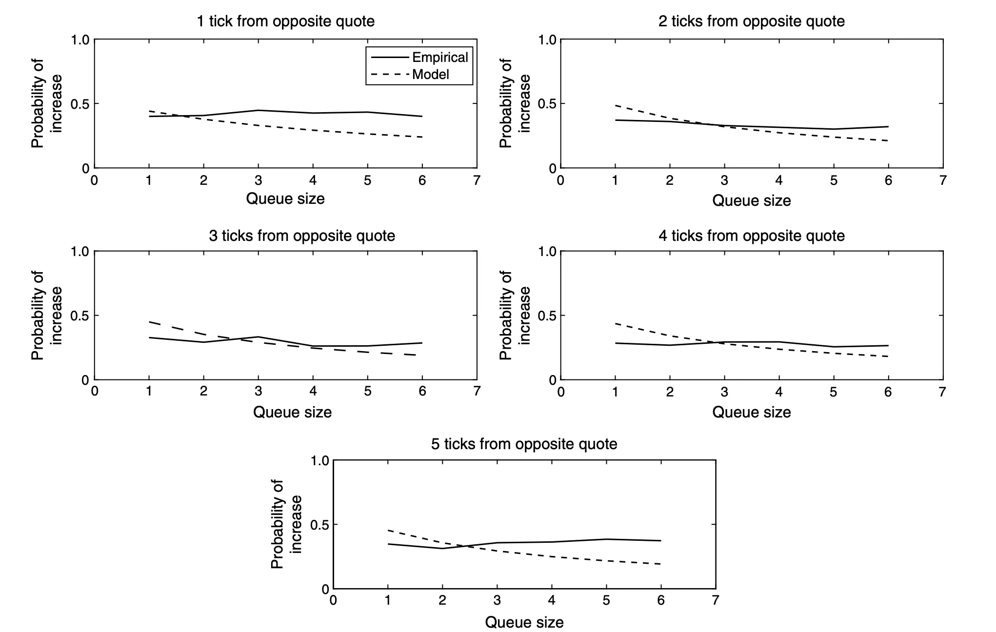
Additionally, the MMRup cap is necessary because the model tends to be conservatively estimated, often ignoring the positive impact of key price points and key bid or ask levels on the order book. Some studies from CME (see Figure 2) illustrate this effect more accurately.

The IMR (Initial Margin Rate) is typically associated with the leverage and liquidity of the underlying asset. Therefore, it often requires dynamic adjustment based on factors such as position size. It can be defined as:

IMR = max(r, w(rMMR))

Here, the IMR corresponds to the initial margin rate r mentioned in Section 2.1. The function w(rMMR) offers more flexibility. For example, if the exchange considers its liquidity to be stable, it can apply a simple adjustment such as: w(rMMR)=1.3×rMMR.

This approach provides a pragmatic way to dynamically adjust margin rates, ensuring that the IMR reflects current market conditions and liquidity levels. This makes the system more adaptive compared to fixed margin rules, benefiting both users and the exchange through effective risk management.

An approximate solution for k

The parameter k serves as a global setting for each specific asset (symbol) and does not need to account for existing orders or open positions. In principle, the larger the value of k, the more positions a user can open. However, there is a critical constraint: the margin required for the maximum allowable position must not exceed the total capital multiplied by the IMR.

To simplify, let’s assign the maximum allowable position formula to a variable v:

v = k ∗ ln(C/(p ∗ r ∗ k) + 1)

The actual leverage must be less than or equal to the reciprocal of the utilized margin:

v/(C/p) <= 1/max(r, f (v, rMMR))

Let’s introduce a new variable y to replace C (capital) and p (price) for simplification:

y = C/p

we get:

v <= y/max(r, f (v, rMMR))

Except for extremely small positions, 1.3 × rMMR (a simplified adjustment using f(pos,rMMR) is generally less than r. For smaller positions, the margin required becomes negligible, so such scenarios are not a concern for our risk model. Similarly, since MMRup sets an upper limit, it can also be ignored in this context.

Thus, we only need to consider the smallest possible value for 1/IMR. The inequality can therefore be simplified as:

v <= y/(1.3 ∗ f (position)/p)

This inequality demonstrates the relationship between the maximum allowable position and actual leverage.

Unlike other variables, position and R have a clearly defined inverse relationship. Therefore, the MMR derived from R can also have an inverse proportional relationship with position, and MMR can be expressed as follows:

MMR = para1 + para2/position

At this point, to assume that the MMR under low positions aligns with the traditional form (half of the inverse of leverage), the formula can be written as:

MMR = 1/(2 ∗ maxleverage) ∗ (1 + pos/position)

Now we attempt to find the limit of k, then r in formula (3) becomes 1/maxleverage.

And, substituting the variables, the inequality (18) can become:

We observe that y (determined by the user’s capital) theoretically should not affect the value of k. Thus, k is primarily dependent on position. Although the minimum value of k varies with changes in y, the objective is to identify the smallest possible minimum across all conditions. This ensures that the opening of positions remains safe under any scenario.

Here, y/(k*r) can still be substituted by a variable, but the equation remains complex and difficult to solve analytically. Some extensive approximation experiments and iterative simulations reveal that k converges to a very simple expression(but the calculation of k is a significant undertaking, so it will not be elaborated on in detail here):

k <= e ∗ position

By adjusting the values of k or position, we can achieve the effect that when the amount of funds or the number of open positions is not large, users can open up to C/(p∗r). Otherwise, they will be restricted. The size of the quantity and the degree of limitation are both controlled by k and position. Therefore, different cryptocurrencies often correspond to different k values.

The above is a brief introduction to KuCoin’s cross-margin risk limit system. The advantages of this design and its user-friendliness are self-evident.

In KuCoin’s cross-margin system, aside from risk limits, other elements such as risk ratios and order margin utilization are also dynamically managed using the mark price. This dynamic management not only maximizes the release of users’ margin but also integrates seamlessly with the new risk limit framework, enhancing system efficiency and user experience.

figure 1:

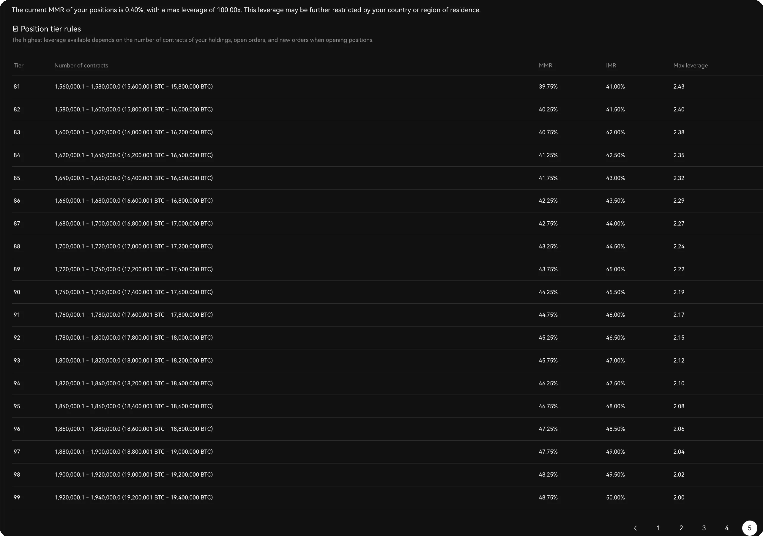
figure 2:

1. “A Stochastic Model for Order Book Dynamics” by Rama Cont, Sasha Stoikov, and Rishi Talreja, Operations Research, Volume 58, Issue 3, in 2010.
2. “Forecasting Initial Margin Requirements – A Model Evaluation” , Journal of Financial Markets (Volume 40, 2018)
3. Alfonsi, A., A. Schied, A. Schulz. 2010. Optimal execution strategies in limit order books with general shape functions. Quant. Finance 10(2).